The concepts behind the algorithm

This guide provides an intuitive description of the steps followed by SCIMES to identify structures within a dataset. The full formalism is reported in <SCIMES paper link>.

Which dataset to use?

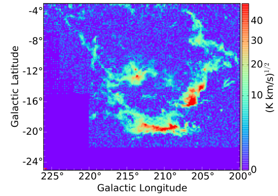
SCIMES can be applied to position-position-velocity (PPV) data cubes, position-position-position simulations or position-position images. For this example we use the PPV data cube of the Orion-Monoceros complex imaged in 12CO(1-0) by Wilson et al. 2005, A&A, 430, 523W whose presents a spatial and spectral resolution of ~ 1 pc (at an average distance to the complex of 450 pc) and 0.65 km/s, respectively. The figure shows the square-root of the integrated intensity map of the dataset.

Building the dendrogram

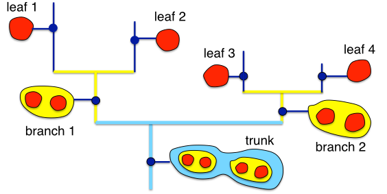
A dendrogram is a tree that represents the hierarchical structure in the data (Rosolowsky et al. 2008, ApJ, 679, 1338R; see also the description for the astrodendro algorithm core). It is composed of two types of structures: branches, which are structures which split into multiple sub-structures, and leaves, which are structures that have no sub-structure (i.e. local maxima). The trunk is a super-structure that has no parent structure, and contains all other structures. In the Orion-Monoceros dataset, branches represent potential Giant Molecular Clouds (GMCs), leaves are essentially clumps within the GMCs, and the trunk can be considered as the full star forming complex. In the figure, stronger connection between the leaves are indicated with yellow lines, while weaker with cyan lines.

A dendrogram as a graph

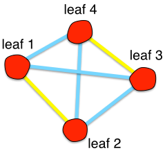
How can we identify relevant objects within the dendrogram? We need first to abstract the dendrogram as a graph. A graph is a collection of objects (nodes) which possess certain relations. These relations are represented by edges between the nodes whose weight indicate the strength of the relations. A dendrogram can be abstract into a graph by considering the “leaves” as graph “nodes”. Every leaf is connected to another leaf in the dendrogram at a given hierarchical level. “Edges” are represented by the highest structure of the dendrogram that contains the two leaves considered. The figure follows the same color convention as the previous one.

From the graph to the affinity matrix

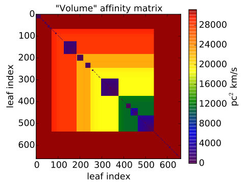
Each edge weight can be collected into an affinity matrix. In a PPV cube, edges are 3D structures (isosurfaces) that possess several physical properties. We define an edge weight (or affinity) as the inverse of a certain isosurface property. In this case we use the “PPV volume”, defined as the product between the area from the effective radius and the velocity dispersion of the isosurfaces. The larger the volume, the lower the affinity, and the lower the possibility for two clumps to belong to same cloud. By default, SCIMES performs the segmentation based on the “volume”, “flux”, or an aggregate version of the two matrices. These properties can also be defined by their physical version once distances are provided.

Cutting the graph through the Spectral Clustering

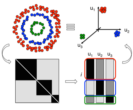
The Spectral Clustering approach translates the ISM property encoded within the matrix into a Euclidean space where the clustering properties of the dendrogram are enhanced. To do this the first k eigenvectors of the affinity matrix are defined (spectral embedding). k defines also the dimensionality of the clustering space and the number of clusters to search. Afterwards, SCIMES automatically finds the best arrangement of leaves into clusters and the best number of clusters, i.e. GMCs. In the figure, a concentric distribution of objects is shown. Objects with the same color have higher affinity (i.e. their connection is stronger). However they cannot be clustered using a Euclidean distance-based algorithm. The spectral clustering transforms all affinity information to the clustering space via spectral embedding of the affinity matrix.

Clustered dendrogram

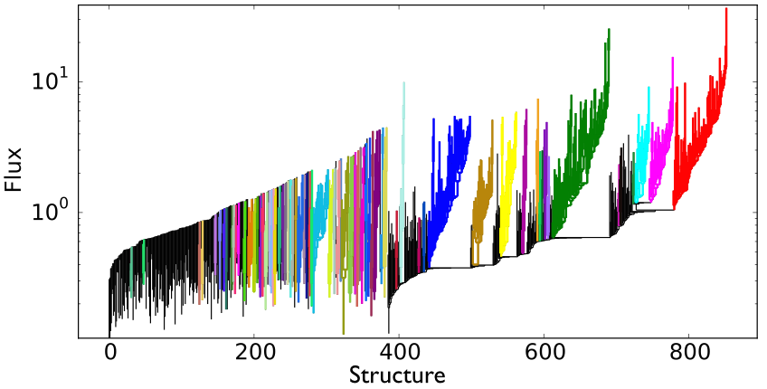
The figure shows the final product of SCIMES: the clustered dendrogram. Each color indicates a relevant branch (i.e. cluster) within the dendrogram, according to the chosen affinity criterion. In this case, the clusters are selected based on their similar maximal volume. Affinity criteria can be based upon virtually any observable property of the ISM.

Giant Molecular Clouds in Orion-Monoceros

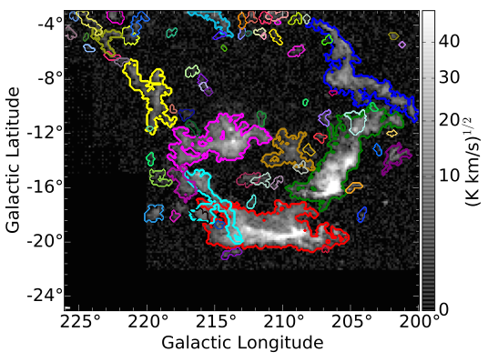
The relevant branches of the Orion-Monoceros associated dendrogram correspond to the notable GMCs of the complex: Orion A (red), Orion B (green), Monoceros (magenta), the Northern Filament (blue), NGC2149 (cyan), the Crossbones (yellow), the Scissors (purple). SCIMES correctly identifies them without over-dividing the molecular emission.